


Next: Correlated Sampling in a
Up: CORRELATED SAMPLING MONTE CARLO
Previous: Numerical Examples
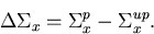
Correlated sampling techniques force all the histories corresponding to the
perturbed system to follow the same transition
points in phase space as the unperturbed histories. Appropriate weight
factors are then used to adjust the particle
weights at the transition points. This can be explained
mathematically by looking at the integral form of the neutron transport
equation (equation 2.1), expressed in terms of collision density and its
solution by the Neumann series [Spa69, Lux91]. The collision density equation
is given by,
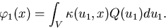
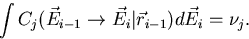
| 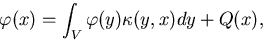 |
(40) |
where x and y are the coordinates of a particle in the six-dimensional phase
space,  is the transport kernel from y to x,
  is the
collision density of particles entering a collision in x, and Q(x) is the
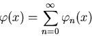
external particle source in x. The Neumann series solution of equation
(3.8) is given by,
is the
collision density of particles entering a collision in x, and Q(x) is the
external particle source in x. The Neumann series solution of equation
(3.8) is given by,
|  |
(41) |
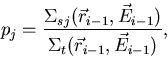
where  is the probability that a particle entering into a
collision at
is the probability that a particle entering into a
collision at  with energy
  will appear at
 with energy
  ,
,
|  |
(42) |
Here
| 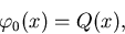 |
(43) |
is the direct source contribution term.
For n = 1 we get the once-collided term,
|  |
(44) |
Similarly for n = 2,3... etc. the twice, thrice ... etc. collided terms can be
found. The transport kernel is expressed in
terms of the product
of a
collision kernel, C(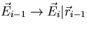 ), and a translation kernel,
T(
), and a translation kernel,
T(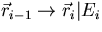 ),
as shown below,
),
as shown below,
|  |
(45) |
or,
|  |
(46) |
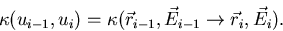
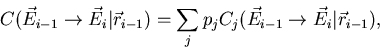
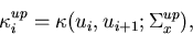
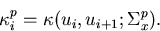
The kernel Ci-1 denotes the probabilities of particles that are coming out of a collision in
with direction  and energy Ei, i.e., =
 . The collision kernel can be represented explicitly as,
|  |
(47) |
where pj denotes the probability of scattering collision of type j, and
Cj is the corresponding collision kernel. Each Cj can be
normalized to the mean number of secondaries,  , per event,
|  |
(48) |
For elastic scattering events, = 1; for fission > 1. The
probabilities pj can be written as,
|  |
(49) |
where  is the macroscopic scattering cross section for
scattering type j.
is the macroscopic scattering cross section for
scattering type j.
The kernel Ti-1 represents the probability for the transport of particles from to
the next
collision in . For example, if  ,the total macroscopic cross section at (
 ), is
spatially constant along the direction
), is
spatially constant along the direction  then,
then,
|  |
(50) |
where d is the distance from to .
To develop expressions for correlated sampling tracking, we will denote
the transport kernel of the unperturbed system by,
|  |
(51) |
and that for the perturbed system by,
|  |
(52) |
 and
and  denote a generic cross section for the
unperturbed
and the perturbed systems, respectively, and the perturbation in cross section
can be expressed as,
denote a generic cross section for the
unperturbed
and the perturbed systems, respectively, and the perturbation in cross section
can be expressed as,
|  |
(53) |
Now the collision densities for the unperturbed and the perturbed systems are
respectively,
| 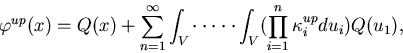 |
(54) |
and
|  |
(55) |
The difference between the two collision densities is a function of the cross
section change  . As shown before, independent simulation of the
unperturbed and perturbed systems and straightforward subtraction of the
results is not sufficient for calculating perturbation effects, especially for
small
perturbations. In the correlated sampling method, the perturbed histories are
forced to
follow the same trajectories as the unperturbed histories including the same
transition points in phase space
[Rie84]. A weight factor is used for the perturbed histories to account for the
resulting biasing due to the forced transition. The weight factor for the
perturbed system is given by,
. As shown before, independent simulation of the
unperturbed and perturbed systems and straightforward subtraction of the
results is not sufficient for calculating perturbation effects, especially for
small
perturbations. In the correlated sampling method, the perturbed histories are
forced to
follow the same trajectories as the unperturbed histories including the same
transition points in phase space
[Rie84]. A weight factor is used for the perturbed histories to account for the
resulting biasing due to the forced transition. The weight factor for the
perturbed system is given by,
| 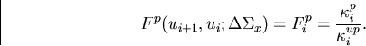 |
(56) |
Now the perturbation effect is given by,
| ![\begin{displaymath}
\sum_{n=1}^{\infty}\int_V\cdot\cdot\cdot\cdot\cdot\int_V(\pr...
...=0}^n{F^p_i}
-1){[\prod_{i=1}^n{\kappa_i^{up}{du_i}}{Q(u_1)}]}.\end{displaymath}](img132.gif) |
(57) |
We notice in the expression for  that the summation
expression for the
unperturbed collision density,
that the summation
expression for the
unperturbed collision density,  , has been multiplied by the
weight factor
, has been multiplied by the
weight factor

 is tallied
at each collision point and contributes to the calculation of the perturbation.
is tallied
at each collision point and contributes to the calculation of the perturbation.
Next: Correlated Sampling in a
Up: CORRELATED SAMPLING MONTE CARLO
Previous: Numerical Examples
Amitava Majumdar
9/20/1999